Cassandra is an open source, distributed database. It’s useful for managing large quantities of data across multiple data centers as well as the cloud.
Cassandra data model
Cassandra’s data model consists of keyspaces, column families, keys, and columns. The table below compares each part of the Cassandra data model to its analogue in a relational data model.
| Cassandra Data Model | Relational Data Model |
|---|---|
| Keyspace | Database |
| Column Family | Table |
| Partition Key | Primary Key |
| Column Name/Key | Column Name |
| Column Value | Column Value |
How Cassandra organizes data
Cassandra organizes data into partitions. Each partition consists of multiple columns. Partitions are stored on a node. Nodes are generally part of a cluster where each node is responsible for a fraction of the partitions.
When inserting records, Cassandra will hash the value of the inserted data’s partition key; Cassandra uses this hash value to determine which node is responsible for storing the data.
Where are the rows?
Cassandra is a column data store, meaning that each partition key has a set of one or more columns. Let’s say we have a list of fruits:
- [Apple, Banana, Orange, Pear]
We create a column family of fruits, which is essentially the same as a table in the relational model. Inside our column family, Cassandra will hash the name of each fruit to give us the partition key, which is essentially the primary key of the fruit in the relational model.
Now things start to diverge from the relational model. Cassandra will store each fruit on its own partition, since the hash of each fruit’s name will be different. Because each fruit has its own partition, it doesn’t map well to the concept of a row, as Cassandra has to issue commands to potentially four separate nodes to retrieve all data from the fruit column family.
We’ll get into more details later, but for now it’s enough to know that for Cassandra to look up a set of data (or a set of rows in the relational model), we have to store all of the data under the same partition key. To summarize, rows in Cassandra are essentially data embedded within a partition due to the fact that the data share the same partition key.
Data model goals
- Spread data evenly around the cluster. Paritions are distributed around the cluster based on a hash of the partition key. To distribute work across nodes, it’s desirable for every node in the cluster to have roughly the same amount of data.
- Minimize the number of partitions read. Partitions are groups of columns that share the same partition key. Since each partition may reside on a different node, the query coordinator will generally need to issue separate commands to separate nodes for each partition we query.
- Satisfy a query by reading a single partition. This means we will use roughly one table per query. Supporting multiple query patterns usually means we need more than one table. Data duplication is encouraged.
Components of the Cassandra data model
Column family
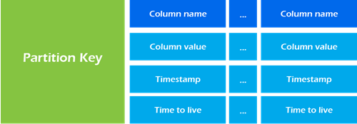
Column families are established with the CREATE TABLE command. Column families are represented in Cassandra as a map of sorted maps. The partition key acts as the lookup value; the sorted map consists of column keys and their associated values.
Map<ParitionKey, SortedMap<ColumnKey, ColumnValue>>Partition key
The partition key is responsible for distributing data among nodes. A partition key is the same as the primary key when the primary key consists of a single column.
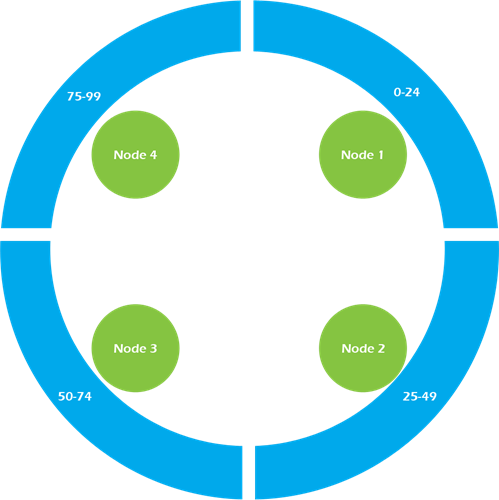
Partition keys belong to a node. Cassandra is organized into a cluster of nodes, with each node having an equal part of the partition key hashes.
Imagine we have a four node Cassandra cluster. In the example cluster below, Node 1 is responsible for partition key hash values 0-24; Node 2 is responsible for partition key hash values 25-49; and so on.
Replication factor
Depending on the replication factor configured, data written to Node 1 will be replicated in a clockwise fashion to its sibling nodes. So in our example above, assume we have a four-node cluster with a replication factor of three. When we insert data with a partition key of 23, the data will get written to Node 1 and replicated to Node 2 and Node 3. When we insert data with a partition key of 88, the data will get written to Node 4 and replicated to Node 1 and Node 2.
Compound key
Compound keys include multiple columns in the primary key, but these additional columns do not necessarily affect the partition key. A partition key with multiple columns is known as a composite key and will be discussed later.
Let’s borrow an example from Adam Hutson’s excellent blog on Cassandra data modeling. Consider a Cassandra database that stores information on CrossFit gyms. One property of CrossFit gyms is that each gym must have a unique name i.e. no two gyms are allowed to share the same name.
The table below is useful for looking up a gym when we know the name of the gym we’re looking for.
CREATE TABLE crossfit_gyms (
 gym_name text,
 city text,
 state_province text,
 country_code text,
 PRIMARY KEY (gym_name)
);
Now suppose we want to look up gyms by location. If we use the crossfit_gyms table, we’ll need to iterate over the entire result set. Instead, we’ll create a new table that will allow us to query gyms by country.
CREATE TABLE crossfit_gyms_by_location (
 country_code text,
 state_province text,
 city text,
 gym_name text,
 PRIMARY KEY (country_code, state_province, city, gym_name)
);
Note that only the first column of the primary key above is considered the partition key; the rest of columns are clustering keys. This means that while the primary key represents a unique gym record/row, all gyms within a country reside on the same partition. So when we query the crossfit_gyms_by_location table, we receive a result set consisting of every gym sharing a given country_code. While useful for searching gyms by country, using this table to identify gyms within a particular state or city requires iterating over all gyms within the country in which the state or city is located.
Clustering key
Clustering keys are responsible for sorting data within a partition. Each primary key column after the partition key is considered a clustering key. In the crossfit_gyms_by_location example, country_code is the partition key; state_province, city, and gym_name are the clustering keys. Clustering keys are sorted in ascending order by default. So when we query for all gyms in the United States, the result set will be ordered first by state_province in ascending order, followed by city in ascending order, and finally gym_name in ascending order.
Order by
To sort in descending order, add a WITH clause to the end of the CREATE TABLE statement.
CREATE TABLE crossfit_gyms_by_location (
 country_code text,
 state_province text,
 city text,
 gym_name text,
 PRIMARY KEY (country_code, state_province, city, gym_name)
) WITH CLUSTERING ORDER BY (state_province DESC, city ASC, gym_name ASC);
The result set will now contain gyms ordered first by state_province in descending order, followed by city in ascending order, and finally gym_name in ascending order. You must specify the sort order for each of the clustering keys in the ORDER BY statement. The partition key is not part of the ORDER BY statement because its values are hashed and therefore won’t be close to each other in the cluster.
Composite key
Composite keys are partition keys that consist of multiple columns. The crossfit_gyms_by_location example only used country_code for partitioning. The result is that all gyms in the same country reside within a single partition. This can lead to wide rows. In the case of our example, there are over 7,000 CrossFit gyms in the United States, so using the single column partition key results in a row with over 7,000 combinations.
To avoid wide rows, we can move to a composite key consisting of additional columns. If we change the partition key to include the state_province and city columns, the partition hash value will no longer be calculated off only country_code. Now, each combination of country_code, state_province, and city will have its own hash value and be stored in a separate partition within the cluster. We accomplish this by nesting parenthesis around the columns we want included in the composite key.
CREATE TABLE crossfit_gyms_by_city (
 country_code text,
 state_province text,
 city text,
 gym_name text,
 opening_date timestamp,
 PRIMARY KEY ((country_code, state_province, city), opening_date, gym_name)
) WITH CLUSTERING ORDER BY ( opening_data ASC, gym_name ASC );
Notice that we are no longer sorting on the partition key columns. Each combination of the partition keys is stored in a separate partition within the cluster.
A note about querying clustered composite keys
When issuing a CQL query, you must include all partition key columns, at a minimum. You can then apply an additional filter by adding each clustering key in the order in which the clustering keys appear. Below you can see valid queries and invalid queries from our crossfit_gyms_by_city example.
Valid queries:
SELECT \* FROM crossfit_gyms_by_city WHERE country_code = 'USA' and state_province = 'VA' and city = 'Arlington'SELECT \* FROM crossfit_gyms_by_city WHERE country_code = 'USA' and state_province = 'VA' and city = 'Arlington' and opening_date < '2015-01-01 00:00:00+0200'Invalid queries:
SELECT \* FROM crossfit_gyms_by_city WHERE country_code = 'USA' and state_province = 'VA'SELECT \* FROM crossfit_gyms_by_city WHERE country_code = 'USA' and state_province = 'VA' and city = 'Arlington' and gym_name = 'CrossFit Route 7'The first invalid query is missing the city partition key column. The second invalid query uses the clustering key gym_name without including the preceding clustering key opening_date.
The reason the order of clustering keys matters is because the clustering keys provide the sort order of the result set. Because of the clustering key’s responsibility for sorting, we know all data matching the first clustering key will be adjacent to all other data matching that clustering key.
In our example, this means all gyms with the same opening date will be grouped together in alphabetical order. Gyms with different opening dates will appear in temporal order.
Because we know the order, CQL can easily truncate sections of the partition that don’t match our query to satisfy the WHERE conditions pertaining to columns that are not part of the partition key. However, because the clustering key gym_name is secondary to clustering key opening_date, gyms will appear in alphabetical order only for gyms opened on the same day (within a particular city, in this case). Therefore, we can’t specify the gym name in our CQL query without first specifying an opening date.
Internal data structure
If we create a column family (table) with CQL:
CREATE TABLE crossfit_gyms (
 gym_name text PRIMARY KEY,
 country_code text,
 state_province text,
 city text
);
And insert a row:
INSERT INTO crossfit_gyms (country_code, state_province, city, gym_name) VALUES ('USA', 'CA', 'San Francisco', 'San Francisco CrossFit');Assuming we don’t encode the data, it is stored internally as:
Partition Key: San Francisco CrossFit
=>(column=, value=, timestamp=1374683971220000)
=>(column=city, value='San Francisco', timestamp=1374683971220000)
=>(column=country_code, value='USA', timestamp=1374683971220000)
=>(column=state_province, value='CA', timestamp=1374683971220000)
You can see that the partition key is used for lookup. In this case the first column is also the partition key, so Cassandra does not repeat the value. The next three columns hold the associated column values.
If we use a composite key, the internal structure changes a bit. Let’s start with a general example borrowed from Teddy Ma’s step-by-step guide to learning Cassandra.
CREATE TABLE example (
partitionKey1 text,
partitionKey2 text,
clusterKey1 text,
clusterKey2 text,
normalField1 text,
normalField2 text,
PRIMARY KEY (
(partitionKey1, partitionKey2),
clusterKey1, clusterKey2
)
);
And insert a row:
INSERT INTO example (
partitionKey1,
partitionKey2,
clusterKey1,
clusterKey2,
normalField1,
normalField2
) VALUES (
'partitionVal1',
'partitionVal2',
clusterVal1',
'clusterVal2',
'normalVal1',
'normalVal2');
This data is stored internally as:
RowKey: partitionVal1:partitionVal2
=> (column=clusterVal1:clusterVal2:, value=, timestamp=1374630892473000)
=> (column=clusterVal1:clusterVal2:normalfield1, value=6e6f726d616c56616c31, timestamp=1374630892473000)
=> (column=clusterVal1:clusterVal2:normalfield2, value=6e6f726d616c56616c32, timestamp=1374630892473000)
The composite key columns are concatenated to form the partition key (RowKey). The clustering keys are concatenated to form the first column and then used in the names of each of the following columns that are not part of the primary key. The actual values we inserted into normalField1 and normalField2 have been encoded, but decoding them results in normalValue1 and normalValue2, respectively.
Now we can adapt this to our CrossFit example.
CREATE TABLE crossfit_gyms_by_state (
 country_code text,
 state_province text,
 city text,
 gym_name text,
 opening_date timestamp,
 street text,
 PRIMARY KEY (
 (country_code, state_province),
 city, gym_name
 )
);
And insert a row:
INSERT INTO crossfit_gyms_by_state (
 country_code,
 state_province,
 city,
 gym_name,
 opening_date,
 street
)
VALUES (
 'USA',
 'CA',
 'San Francisco',
 'San Francisco CrossFit',
 '2015-01-01 00:00:00+0200',
 '1162A Gorgas Ave');
For the sake of readability, I won’t encode the values of the columns. The internal structure is approximately:
Partition Key: USA:CA
=>(column='San Francisco':'San Francisco CrossFit', value=, timestamp=1374683971220000)
=>(column='San Francisco':'San Francisco CrossFit':'opening_date', value='2015-01-01 00:00:00+0200', timestamp=1374683971220000)
=>(column='San Francisco':'San Francisco CrossFit':'street', value='1162A Gorgas Ave', timestamp=1374683971220000)Finally, we’ll show how Cassandra represents sets, lists, and maps internally. Once again, we’ll use an example from Teddy Ma’s step-by-step guide to learning Cassandra.
CREATE TABLE example (
 key1 text PRIMARY KEY,
 map1 map<text,text>,
 list1 list<text>,
 set1 set<text>
);
Insert a row:
INSERT INTO example (
 key1,
 map1,
 list1,
 set1
) VALUES (
 'john',
 {'patricia':'555-4326','doug':'555-1579'},
 ['doug','scott'],
 {'patricia','scott'}
);
Internally:
RowKey: john
=> (column=, value=, timestamp=1374683971220000)
=> (column=map1:doug, value='555-1579', timestamp=1374683971220000)
=> (column=map1:patricia, value='555-4326', timestamp=1374683971220000)
=> (column=list1:26017c10f48711e2801fdf9895e5d0f8, value='doug', timestamp=1374683971220000)
=> (column=list1:26017c12f48711e2801fdf9895e5d0f8, value='scott', timestamp=1374683971220000)
=> (column=set1:'patricia', value=, timestamp=1374683971220000)
=> (column=set1:'scott', value=, timestamp=1374683971220000)
To store maps, Cassandra adds a column for each item in the map. The column name is a concatenation of the the column name and the map key. The value is the key’s value.
To store lists, Cassandra adds a column for each entry in the list. The column name is a concatenation of the the column name and a UUID generated by Cassandra. The value is the value of the list item.
To store sets, Cassandra adds a column for each entry. The column name is a concatenation of the the column name and the entry value. Cassandra does not repeat the entry value in the value, leaving it empty.
Conclusion
You now have enough information to begin designing a Cassandra data model. Remember to work with the unstructured data features of Cassandra rather than against them. Designing a data model for Cassandra can be an adjustment coming from a relational database background, but the ability to store and query large quantities of data at scale make Cassandra a valuable tool.
Appendix
Cassandra Features
- Continuous availability. The peer-to-peer replication of data to nodes within a cluster results in no single point of failure. This is true even across data centers.
- Linear performance when scaling nodes in a cluster. If three nodes are achieving 3,000 writes per second, adding three more nodes will result in a cluster of six nodes achieving 6,000 writes per second.
- Tunable consistency. If we want to replicate data across three nodes, we can have a replication factor of three, yet not necessarily wait for all three nodes to acknowledge the write. Data will eventually be written to all three nodes, but we can acknowledge the write after writing the data to one or more nodes without waiting for the full replication to finish.
- Flexible data model. Every row can have a different number of columns with support for many types of data.
- Query language (CQL) with a SQL-like syntax.
- Support for Java Monitoring Extensions (JMX). Metrics about performance, latency, system usage, etc. are available for consumption by other applications.
Cassandra Limitations
- No join or subquery support for aggregation. According to Cassandra’s documentation, this is by design, encouraging denormalization of data into partitions that can be queried efficiently from a single node, rather than gathering data from across the entire cluster.
- Ordering is set at table creation time on a per-partition basis. This avoids clients attempting to sort billions of rows at run time.
- All data for a single partition must fit on disk in a single node in the cluster.
- It’s recommended to keep the number of rows within a partition below 100,000 items and the disk size under 100 MB.
- A single column value is limited to 2 GB (1 MB is recommended).
A less obvious limitation of Cassandra is its lack of row-level consistency. Modifications to a column family (table) that affect the same row and are processed with the same timestamp will result in a tie.
In the event of a tie Cassandra follows two rules:
- Deletes take precedence over inserts/updates.
- If there are two updates, the one with the lexically larger value wins.
This means for inserts/updates, Cassandra resolves row-level ties by comparing values at the column (cell) level, writing the greater value. This can result in one update modifying one column while another update modifies another column, resulting in rows with combinations of values that never existed.